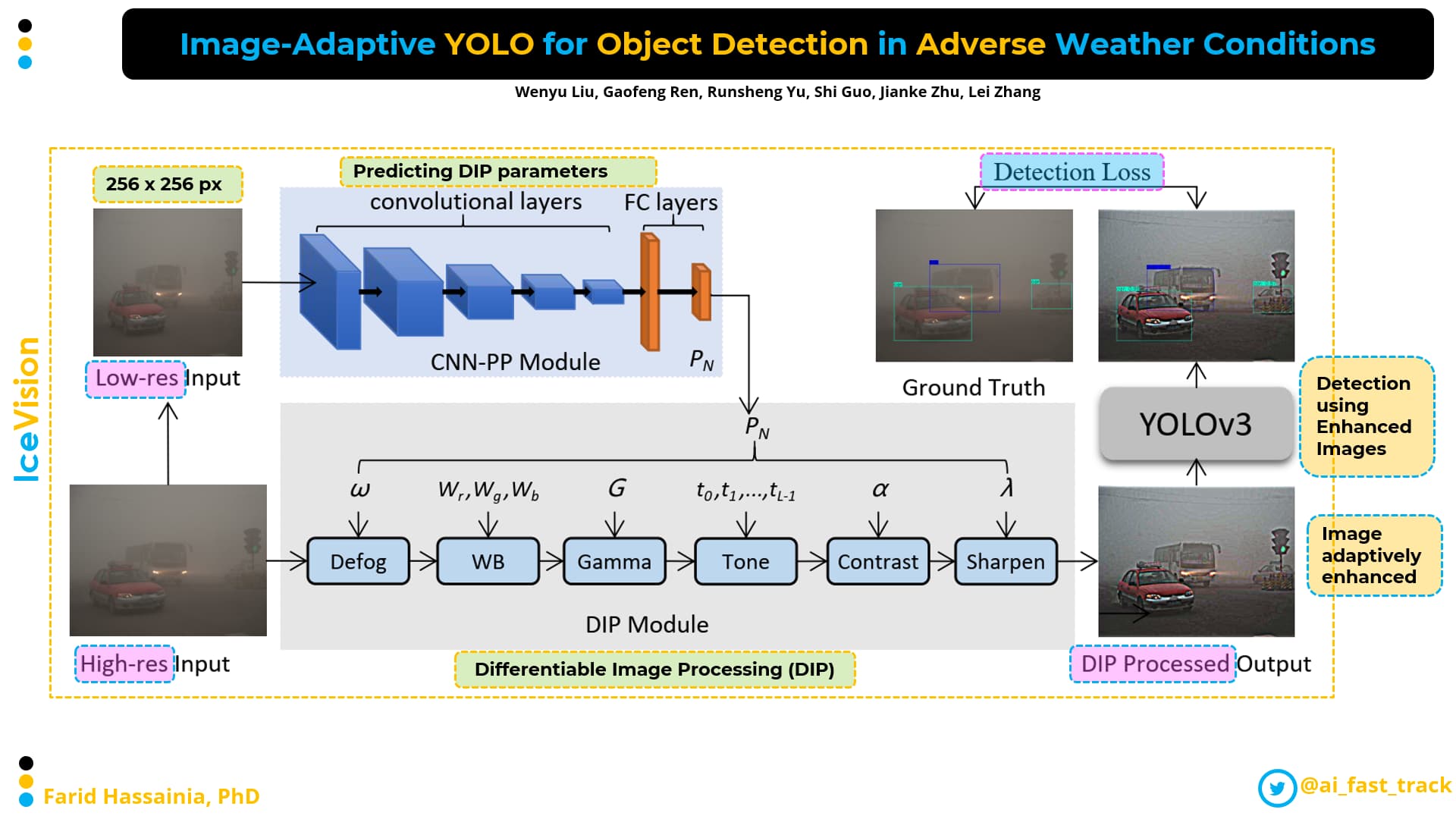
Computer vision applications require lightning-fast inference to process video streams without lag. Traditional two-stage detectors struggle with real-time performance because they separate region proposal from classification. The You Only Look Once framework, universally known as YOLO, changed this dynamic by framing object detection as a single regression problem. Instead of scanning an image multiple times, a single neural network pass predicts bounding boxes and class probabilities simultaneously.
Understanding how these models operate allows developers to deploy high-speed vision systems for surveillance, manufacturing automation, and robotics. This guide breaks down the core architecture, traces the evolution of the model family, provides an implementation blueprint, and tackles common production bottlenecks.
How YOLO Works Under the Hood
The core innovation of the architecture lies in treating image analysis as a holistic regression task rather than a piecemeal classification chore.
When an image enters the network, the model divides the frame into an $S \times S$ grid. If an object's center falls inside a specific grid cell, that cell takes responsibility for detecting it. Each cell predicts multiple bounding boxes alongside confidence scores that reflect how accurately the box fits the target and whether an object actually resides inside it. Further analysis by Bloomberg explores similar perspectives on this issue.
The prediction vector for each bounding box contains coordinates for the center offset, dimensions, and class probabilities. By processing the entire image in a single forward pass, the system bypasses the redundant regional proposal steps used by older architectures.
Multi-Scale Feature Extraction
Modern iterations process images across multiple spatial resolutions simultaneously. Backbone networks extract feature maps at different strides, typically balancing fine-grained spatial details with deep semantic context.
- Small-stride grids: Focus on tiny objects by retaining high-resolution spatial details.
- Medium-stride grids: Handle standard objects requiring a balance of context and localization.
- Large-stride grids: Capture large objects by aggregating wide contextual information across the frame.
Evolution of the YOLO Family
Since its initial release, the architecture has undergone massive structural overhauls. The transition from darknet-based C implementations to native PyTorch libraries opened the door for rapid industrial adoption.
The early versions established real-time baselines, while subsequent updates like Ultralytics YOLO introduced anchor-free prediction, improved loss functions, and modular scaling. Newer iterations incorporate attention-based blocks and expanded capabilities that stretch beyond standard bounding boxes into instance segmentation, pose estimation, and oriented bounding boxes.
Implementing Object Detection in Python
Getting started with a pre-trained model requires minimal boilerplate code thanks to modern Python libraries. You can load a standard model, run inference on a local image file, and inspect the resulting detections with a few lines of code.
from ultralytics import YOLO

# Load a pre-trained medium model
model = YOLO("yolov8m.pt")

# Run inference on an image source
results = model("traffic.jpg", conf=0.4)

# Print detected classes and bounding boxes
for r in results:
    for box in r.boxes:
        class_id = int(box.cls[0])
        confidence = float(box.conf[0])
        print(f"Detected class {class_id} with confidence {confidence:.2f}")
For custom training workflows, organize your dataset into standard directory structures containing image folders and text annotation files matching the normalized bounding box coordinates. You can initialize training via the command line or directly inside a training script by passing your configuration YAML file.
Common Production Mistakes
Deploying vision models to production environments often introduces performance bottlenecks that don't appear in local development notebooks. Avoiding these pitfalls ensures stable performance under heavy workloads.
- Ignoring Hardware Constraints: Running large model variants on resource-constrained edge devices causes frame drops. Always match the model size—such as nano or small variants—to your target hardware capabilities.
- Neglecting Post-Processing Export: Running raw PyTorch weights in production introduces unnecessary latency. Exporting models to optimized runtimes like ONNX or TensorRT significantly accelerates inference speed on CPU and GPU hardware.
- Improper Confidence Thresholds: Setting confidence thresholds too low introduces false positives, while setting them too high causes the model to miss valid targets. Tune your thresholds against validation sets that mirror real-world lighting and angle variations.
For a deeper dive into hardware acceleration and deployment pipelines, consult the Roboflow Computer Vision Guide for end-to-end configuration patterns.
Frequently Asked Questions
What hardware is required to run real-time inference?
Running smaller nano or small variants is feasible on modern multi-core CPUs at reduced frame rates, but production deployments requiring 30+ frames per second typically demand an NVIDIA GPU with TensorRT support.
How do anchor-free models change detection?
Older versions relied on predefined anchor boxes matching specific aspect ratios. Anchor-free architectures predict object centers directly, simplifying training pipelines and improving generalization across unusual object shapes.
Can these models handle tasks other than bounding boxes?
Yes. Modern framework versions support multi-task learning, allowing a single architecture to perform object detection, instance segmentation, pose estimation, and classification simultaneously.
How many images are needed to train a custom detector?
While pre-trained weights reduce data requirements through transfer learning, training a robust custom model typically requires a few hundred to several thousand annotated images per class, depending on background complexity and visual variation.