Finding the optimal mobile phase velocity is essential for maximizing separation efficiency in high-performance liquid chromatography. When you master your flow rate, you sharpen peak shapes, reduce analysis times, and extend column lifetimes. A poorly chosen linear velocity leads to broad peaks, excessive backpressure, and poor resolution that ruins quantitative assays.
Chromatographers frequently rely on the van Deemter equation to locate this balance between mass transfer resistance and longitudinal diffusion. Understanding how particle diameter, column dimensions, and mobile phase viscosity interact allows you to dial in operational parameters with absolute precision. Let's look at the mechanical principles, mathematical formulas, and practical tuning procedures required to reach peak efficiency.
The Van Deemter Equation and Mass Transfer
Theoretical plate height ($H$) serves as the primary metric for column efficiency. The van Deemter equation models how mobile phase linear velocity ($u$) influences this plate height through three distinct chromatographic phenomena: eddy diffusion ($A$), longitudinal diffusion ($B$), and resistance to mass transfer ($C$).
The mathematical representation of the van Deemter relationship is: To read more about the history of this, Associated Press offers an in-depth summary.
$$H = A + \frac{B}{u} + C \cdot u$$
Each term responds differently to changes in flow rate:
- Eddy diffusion ($A$): Independent of velocity, this term accounts for multiple flow paths available to analyte molecules through packed stationary phase particles. Smaller, more uniform particles minimize $A$.
- Longitudinal diffusion ($B$): Inversely proportional to velocity, this term describes analyte molecules diffusing randomly along the column axis from high to low concentration zones. Higher flow rates reduce time for longitudinal spreading.
- Mass transfer resistance ($C$): Directly proportional to velocity, this term measures the time required for analyte molecules to partition between the mobile and stationary phases. Fast flow rates increase mass transfer resistance, causing band broadening.
When you plot plate height against linear velocity, the resulting hyperbola dips to a minimum point. That trough represents the optimal flow rate where overall band broadening is minimized and column efficiency peaks.
Calculating Optimal Linear Velocity
Translating volumetric flow rate ($F$, in mL/min) into linear velocity ($u$, in mm/s) requires accounting for column geometry and total porosity. Using the correct conversion formula prevents you from misjudging efficiency when transferring methods between columns of different inner diameters.
The formula for linear velocity is:
$$u = \frac{L}{t_0}$$
Where $L$ is the column length in millimeters and $t_0$ is the dead time (or void time) in seconds, measured using an unretained marker compound such as uracil or acetone. Alternatively, you can calculate linear velocity from volumetric flow rate using column inner diameter ($d_c$) and total column porosity ($\varepsilon_T$, typically around 0.6 for fully porous particles):
$$u = \frac{4 \cdot F}{\pi \cdot d_c^2 \cdot \varepsilon_T}$$
To determine the sweet spot experimentally, construct a van Deemter plot by injecting a test mix at five distinct flow rates spanning 50% to 200% of your current method's nominal rate. Measure the resulting peak widths at half-maximum, calculate plate count for each run, and plot plate height against flow rate.
Adjusting for Column Particle Dimensions
Particle technology dictates your operational velocity limits. Traditional fully porous particles (3 µm to 5 µm) operate best at moderate velocities because mass transfer resistance increases rapidly in larger packings. Sub-2 µm fully porous particles and superficially porous particles (often called core-shell or superficially porous particles) flatten the $C$-term slope significantly.
Core-shell particles provide shorter diffusion paths inside the particle core, allowing you to run higher flow rates without severe losses in efficiency. When switching from a 5 µm column to a 2.7 µm core-shell column of identical dimensions, you can double your linear velocity while maintaining or even improving separation resolution.
Backpressure scales inversely with the square of particle diameter ($d_p^2$) and directly with column length. Monitoring system pressure limits prevents hardware failure during high-velocity method optimization. Consult Agilent Technologies HPLC Columns or manufacturer specifications to verify maximum pressure ratings before pushing pumps beyond standard operational envelopes.
Common Optimization Mistakes
Chromatographers often make avoidable errors when adjusting flow rates during method development or troubleshooting:
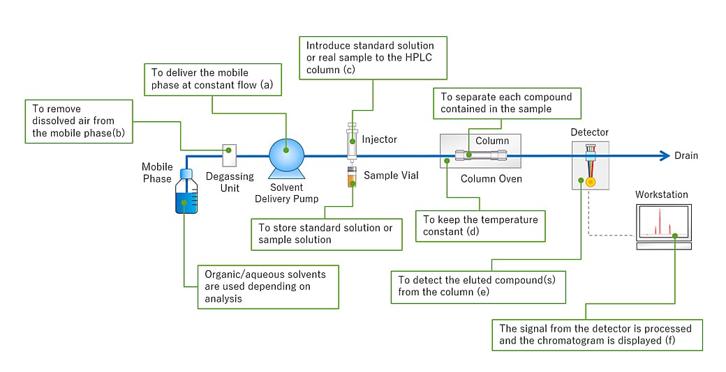
- Ignoring extra-column volume: Tubing that is too wide or long between the injector, column, and detector causes severe band broadening that overshadows improvements gained from optimizing column flow.
- Overlooking mobile phase viscosity: Changing organic modifier ratios alters viscosity, which shifts optimum velocity. Methanol-water mixtures have significantly higher viscosities than acetonitrile-water mixtures, requiring lower flow rates to avoid excessive backpressure.
- Neglecting thermal effects: High flow rates generate frictional heat inside narrow columns. If radial temperature gradients develop, analyte retention times shift and peak splitting occurs.
- Failing to re-optimize gradients: When speeding up an isocratic separation by increasing flow rate, you must scale injection volumes and gradient delay times proportionally to preserve elution profiles.
Frequently Asked Questions
How do I know if my flow rate is too high?
Excessive flow rates manifest as asymmetric peak tailing, split peaks caused by viscous heating, and system pressure alarms. If resolution between early-eluting peaks degrades sharply while retention factors drop below acceptable thresholds, your velocity has exceeded the mass transfer optimum.
Can I change the flow rate without re-validating my method?
According to pharmacopeial guidelines (such as USP chapter 621), you can adjust flow rate proportionally when changing column dimensions or particle sizes, provided you maintain constant linear velocity and resolution criteria. Altering flow rate on an existing, validated method without justification requires re-validation.
Why do sub-2 µm particles require ultra-high pressure systems?
Because particle diameter appears squared in the denominator of the Darcy-Kozeny backpressure equation, cutting particle size in half quadruples the pressure drop across the bed. Conventional HPLC pumps rated at 400 bar cannot deliver the required linear velocity, necessitating UHPLC systems capable of 1000 to 1300 bar.
Does temperature affect the optimal flow rate sweet spot?
Yes. Increasing column oven temperature decreases mobile phase viscosity and enhances analyte diffusion coefficients. This shifts the van Deemter curve downward and moves the minimum to a higher velocity, allowing faster analyses without sacrificing efficiency.


