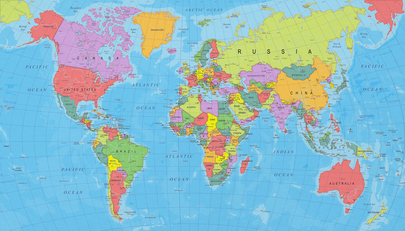
Accessing historical weather records and long-term environmental projections used to mean digging through static spreadsheets or cumbersome command-line archives. Today, tools like NOAA's Climate Data Online and similar spatial interfaces let you query global environmental records directly through interactive maps. You don't need a background in geographic information systems to pull temperature baselines, track precipitation anomalies, or visualize extreme weather frequencies for your exact geographic coordinates.
When you're trying to evaluate local climate exposure or pull environmental metrics for a planning report, static data tables won't cut it. Spatial search tools bridge the gap between raw meteorological records and actionable analysis. Let's look at how these platforms work, how to extract precise insights, and where common analysis pitfalls happen.
Understanding Climate Data Online Spatial Tools
Traditional weather archives store records as tabular time series. While useful for checking specific station readings, tables make spatial patterns invisible. Interactive map search engines overlay meteorological stations, gridded datasets, and observation networks onto dynamic geographic baselines.
When you open a climate mapping tool, you're interacting with three core layers:
- Station metadata layers: Individual weather monitoring posts that track daily or hourly barometric pressure, temperature highs and lows, and rainfall amounts.
- Gridded interpolation models: Modeled surfaces that fill the gaps between physical stations using satellite telemetry and atmospheric physics equations.
- Projection layers: Downscaled climate model outputs projecting temperature and precipitation trends decades into the future under various emissions scenarios.
Instead of typing station IDs or postal codes into a search box, you drop a pin or draw a bounding box over a region. The system queries underlying spatial databases to return records specific to that polygon. That means you can instantly compare a river basin's historical flood records against adjacent upland precipitation trends without manually merging disparate CSV files.
Core Features of Interactive Climate Search Interfaces
Modern climate mapping portals rely on specific filtering and visualization capabilities to handle massive datasets without crashing your browser. Understanding how these features operate helps you pull cleaner data faster.
Spatial Extent and Bounding Controls
You can toggle between continental views down to hyper-local station coordinates. When you zoom in past a certain threshold, minor stations and specialized sensors appear. If you're analyzing urban heat islands, you'll want to isolate urban core stations from rural reference stations to avoid skewed baseline averages.
Temporal Filtering and Normal Periods
Climate analysis requires standardized comparison periods, usually 30-year blocks known as climate normals (such as 1991-2020). Interactive search tools let you slide through temporal windows to check how seasonal norms have shifted over consecutive decades. You aren't just looking at last July's temperature; you're comparing it against the fifty-year distribution for that exact month.
Parameter Selection and Unit Conversion
Raw data feeds often arrive in metric or imperial units depending on the reporting agency. Quality mapping tools include live unit toggles for millimeters to inches, Celsius to Fahrenheit, and station elevation adjustments. You can isolate specific parameters like cooling degree days, consecutive dry days, or maximum single-day precipitation events.
Step-by-Step Guide to Querying Spatial Climate Records
If you want to pull reliable insights without running into data gaps or corrupted exports, follow a structured query workflow.
- Define your geographic boundary: Decide whether you need point data (a single facility or property) or polygon data (a watershed, county, or municipal district). Draw your boundary carefully to exclude irrelevant microclimates, such as mountain peaks that don't reflect valley floor conditions.
- Select your baseline period: Choose your temporal range based on your project requirements. For infrastructure design, use multi-decade normals. For recent anomaly tracking, select the past five to ten years of monthly records.
- Audit station density and missing data: Check the data completeness score for the stations inside your search area. A station with thirty percent missing daily records in summer will distort your drought analysis.
- Export with metadata: Always download the accompanying readme files and station history notes alongside your CSV or GIS shapefile exports. Knowing when a station was relocated or when its instrumentation was upgraded prevents false trend conclusions.
To explore the primary federal archive for these records, visit the NOAA Climate Data Online Portal. For European regional datasets and advanced spatial layers, the Copernicus Climate Change Service provides extensive global reanalysis tools.
Common Pitfalls in Climate Data Analysis
Even with intuitive map interfaces, it's easy to misinterpret environmental records if you skip basic quality checks.
- Ignoring station relocation bias: If a weather station moved two miles uphill or away from an expanding parking lot in 1985, the temperature trend will show an artificial jump or drop. Always check station history logs.
- Confusing weather with climate: A single cold winter in one region doesn't invalidate a fifty-year warming trend. Make sure your temporal queries span sufficient decades to filter out natural year-to-year variability like El Niño cycles.
- Overlooking interpolation error: Gridded datasets estimate conditions between stations using computer models. In topographically complex terrain like mountain ranges or coastal cliffs, these estimates can miss local microclimate variations entirely.
Frequently Asked Questions
What is the difference between station data and gridded climate data?
Station data comes directly from physical thermometers, rain gauges, and anemometers fixed at specific locations. Gridded data uses computer models to interpolate those readings across a continuous spatial grid, filling in the gaps where no physical station exists.
Why do climate normal periods change every ten years?
Meteorological agencies update 30-year climate normals (such as moving from 1981-2010 to 1991-2020) to reflect ongoing shifts in baseline weather patterns. This ensures that when weather forecasters talk about "normal" temperatures, they are referencing recent decades rather than outdated mid-century climates.
Can I export data from interactive climate maps into GIS software?
Most professional mapping portals let you export query results as CSV spreadsheets, GeoJSON files, or shapefiles. You can import these directly into desktop GIS software like QGIS or ArcGIS for advanced spatial modeling.
How do I account for missing data in older historical records?
When historical records have gaps, reliable platforms offer quality-controlled composite datasets or nearest-neighbor imputation models. Always check the metadata flags attached to individual data points to see if a reading was observed or estimated.